
Quick navigation:
Related material:Introduction
Traffic Cellular Automata (TCA) are microscopic traffic simulators that are based on sets of rules that describe the movements of individual vehicles with respect to a grid of cells (i.e., particle hopping models). Reading about it, I became interested in their use and found it worthy to create some rudimentary TCA software myself. The result is a one-dimensional cellular automaton with periodic boundary conditions (i.e., vehicles drive on a unidirectional circular road). Different sets of rules can be chosen and for each set its parameters can be changed at run-time. I also added a traffic light (with cyclical red and green phases) for studying queueing behaviour as well as artificial loop detectors in order to obtain macroscopic measurements (e.g., fundamental diagrams).
The following cellular automata are implemented:
- CA-184 (the deterministic TCA, like Wolfram's rule 184),
- STCA (Nagel-Schreckenberg stochastic traffic cellular automaton),
- STCA-CC (like the STCA but with cruise-control),
- VDR TCA (like the STCA but with velocity-dependent-randomization),
- VDR-CC TCA (like the VDR TCA but with cruise-control),
- Fukui-Ishibashi TCA,
- Takayasu-Takayasu TCA (original),
- Takayasu-Takayasu TCA (modified),
- Time-Oriented CA (TOCA),
- TASEP (totally asymmetric simple exclusion process),
- Cochinos' TCA (a TCA-variant, by Richard Cochinos, I once encountered on the web),
- Emmerich-Rank TCA,
- Helbing-Schreckenberg TCA,
- Brake Light TCA,
- and the Kerner-Klenov-Wolf TCA.
This software is referenced on the Traffic Forum (see section Links, subsection Online Traffic Simulation or Visualization (Java Applets) at item Java (Swing) application for several cellular automata models).
Screenshots
Click on the thumbnails for larger versions.
|
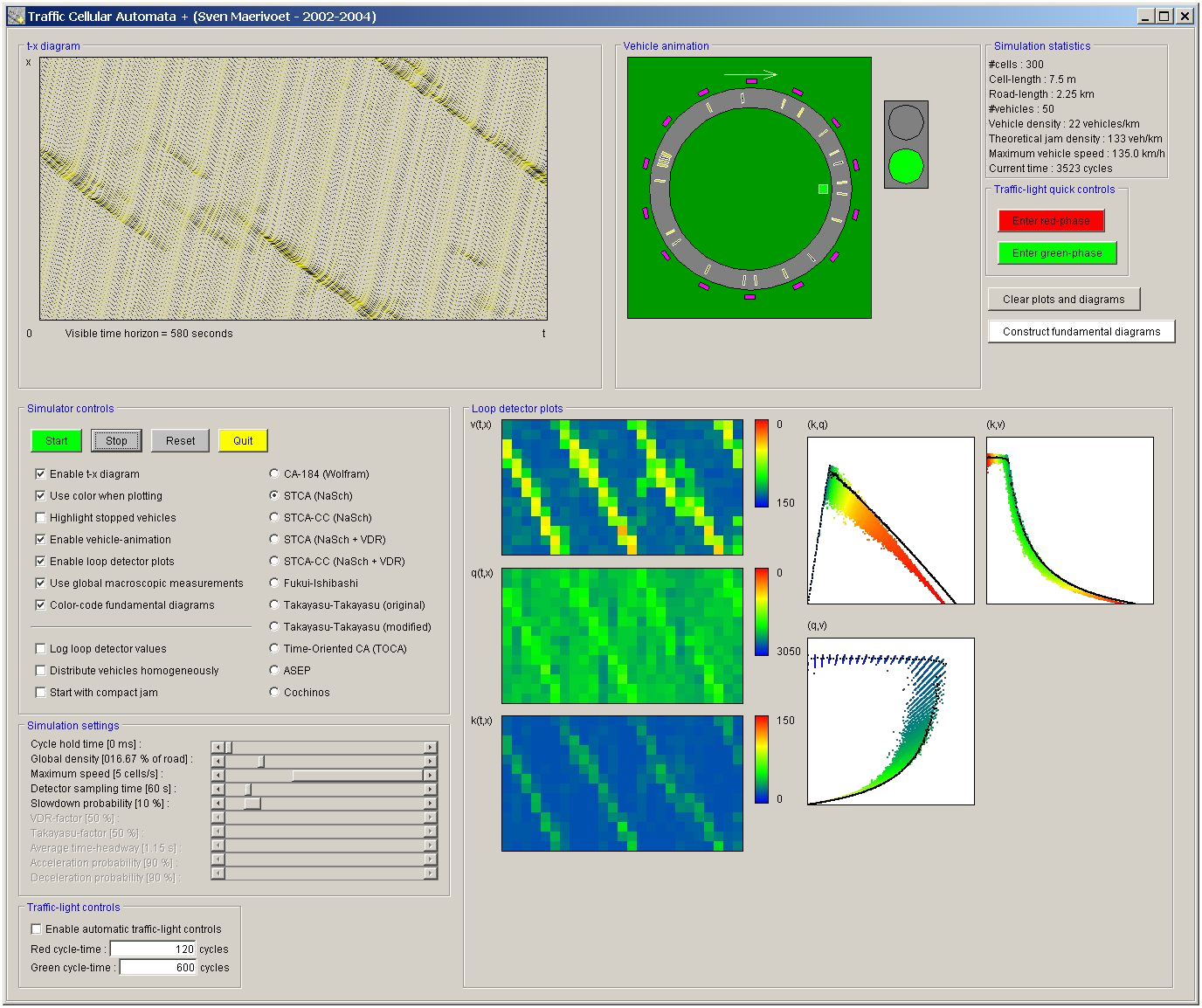
Main graphical user interface This is the huge graphical user interface (it spans approximately 1300x1100 pixels and scrollbars are automatically placed if it doesn't fit on the screen). It consists of several panels : a scrolling t-x diagram, an animation of the road situation, a panel containing some simulation statistics, several simulator controls, scrolling loop detector plots and plots of the fundamental diagrams. |
|
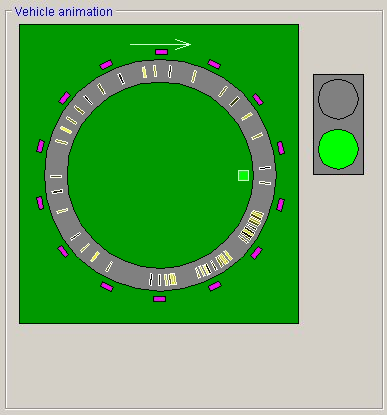
Vehicle animation Looking at a t-x diagram, one can discern the typical back-traveling shockwaves of congestion. But the software also allows one to look at the road situation on which these waves manifest themselves as moving regions of (locally) increased densities. Alongside the road, the positions of all the loop detectors are indicated by small purple boxes. The small green box indicates the position of the traffic light (vehicles travel in a clockwise fashion). |
|
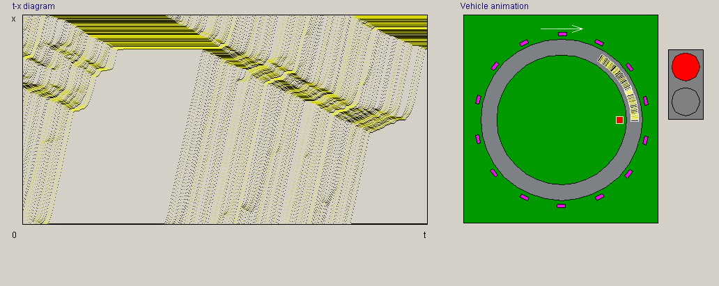
Queueing behind a traffic light The simulator also includes a traffic light for studying queueing behaviour. When the light is red, all vehicles bunch up behind it (which is clearly visible in the animation of the road situation) and the t-x diagram shows a large block of horizontal lines (indicating stopped vehicles). Dissolvement of the queue is also visible when the light turns green again. |
|
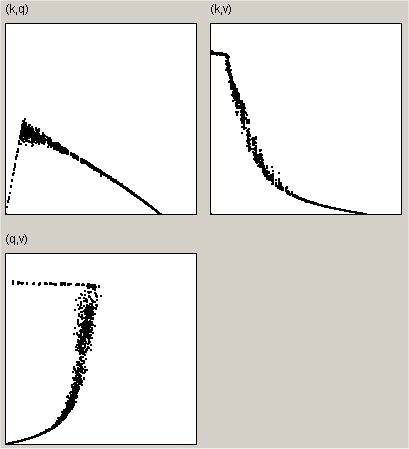
Fundamental diagrams The software has the ability to extract macroscopic flow measurements from several uniformly road-side placed loop detectors which record traffic flow, density and average speed. When these values are pairwise correlated (for identical timestamps), plots of the fundamental diagrams are constructed. There's also the possibility to average measurements from all the loop detectors, resulting in the black fundamental diagrams which relate to the situation on the complete road. |
|
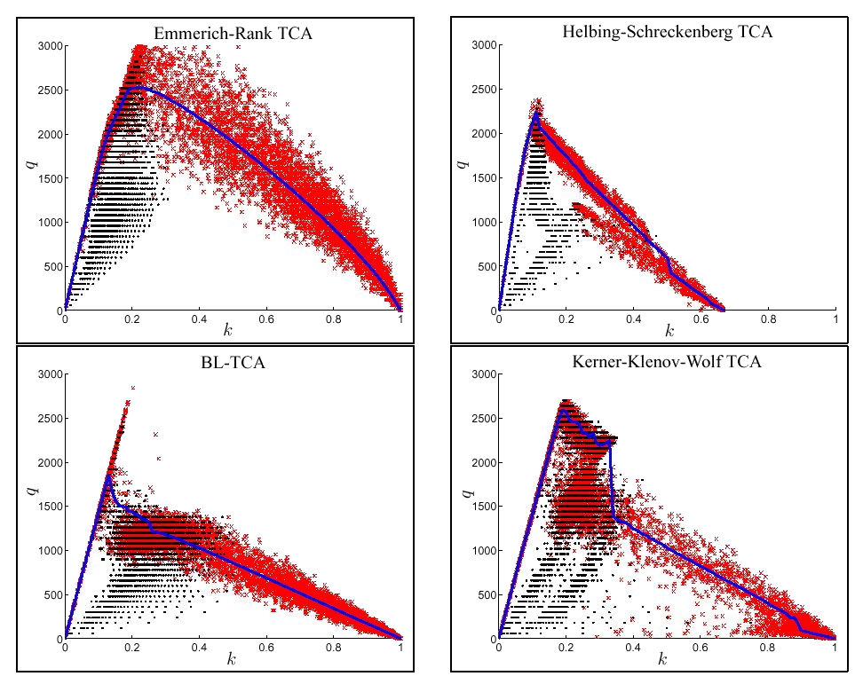
Local and global fundamental diagrams Using MATLAB, we created these graphs showing local and global measurements on the system's lattice, resulting in the well-known (density,flow) fundamental diagrams. The thick blue line is based on global measurements, the red crosses are based on local measurements of one loopdetector that records the density and speed, converting it into a flow value, and the black dots are local measurements of one loopdetector that records the flow and the speed, converting it into a density value. |
Implementation Details
It should be noted that the software is not implemented as an applet but instead as a full Java-application because it uses Swing components that are not standard supported by most browsers (at least not without installing the necessary plugin). The source itself logically consists of three different parts:
- the TCA engine with different rule sets,
- the graphical user interface
- and a whole range of predefined experiments.
TCA engine
The geometrical configuration used in the engine is a unidirectional ring road (i.e., closed boundary conditions) with a single lane. Vehicles are located in cells of 7.5 meter length and can have speeds of 0 to 5 cells/second (which corresponds to a maximal speed of 135 km/h). One iteration in the simulation corresponds to a time step of approximately one second.
A number of artificial loop detectors are uniformly placed alongside the road and aggregate macroscopic traffic measurements (flow, density and space mean speed). Each detector averages over a certain time period and road segment. The measured space mean speed is the average speed of all the vehicles on the road segment during the measurement period. The (local) density is measured the number of vehicles positioned on a specific road segment and the flow is calculated using the fundamental formula : flow = density times speed. Note that it is also possible to calculate these macroscopic quantities in a global manner.
The traffic light is located at the first cell, so stopped vehicles will queue behind the first stopped vehicled (which is then located at this first cell), so their actual positions are the last cells of the closed ring road.
Several rulesets are implemented (they are derived from a base class containing an empty ruleset):
-
CA-184
This deterministic cellular automaton is like the STCA but now the slowdown probability (i.e., the randomization of the vehicles' speeds) is set to zero, like in Wolfram's rule 184.
-
STCA
This is the classical Nagel-Schreckenberg stochastic traffic cellular automaton in which vehicles accelerate gradually until the maximum speed or the space headway with the leading vehicle is reached (which is an upper cut-off). Vehicles slowdown according to a certain probability, decreasing their speed by one (with zero the as the lower limit).
-
STCA-CC
This is the cruise-control variant of the STCA-CC and operates just the same but with one important exception : the randomization of the vehicles' speeds is restricted to slow moving vehicles, i.e., vehicles whose speeds are strictly less than the maximal speed.
-
VDR TCA
The velocity-dependent-randomization traffic cellular automaton is very similar to the STCA, but now there are two probabilities involved : the standard slowdown probability is now used for moving vehicles, the other probability is used for stopped vehicles. This leads to slow-to-start behaviour (and usually one chooses the second probability much higher than the first). The VDR-TCA gives rise to a phase separation in the system: free-flowing traffic coexists with a tight compact jam of stopped vehicles.
-
VDR-CC TCA
This is the cruise-control variant of the VDR TCA and operates just the same but with one important exception : the randomization of the vehicles' speeds is restricted to slow moving vehicles, i.e., vehicles whose speeds are strictly less than the maximal speed.
-
Fukui-Ishibashi TCA
This cellular automaton operates very similar to the STCA, but now the acceleration of a vehicle is direct instead of gradually (with the minimum of the maximal speed and the lead gap as the upper limit). The randomization remains the same.
-
Takayasu-Takayasu TCA (original)
This TCA model is based based upon Takayasu and Takayasu's model (with a maximal speed of 1 cell/s), but we changed the ruleset so that it allows for a higher maximal speed. The model is deterministic, but there is a catch: stopped vehicles are only allowed to accelerate if their space gap is at least two cells. This results in metastable behaviour near the critical density.
-
Takayasu-Takayasu TCA (modified)
This TCA model is based on the previous one, but with the introduction of stochastic noise. Now, a stopped vehicle with at least one empty cell in front of it, can accelerate with a certain probability.
-
Time-Oriented CA (TOCA)
Most traffic cellular automata are space-oriented, which means they consider the absolute size of a gap in front of a vehicle to determine its behaviour. The TOCA however takes into account the current speed of a vehicle and relates this with its driver's reaction time to obtain a safe following distance. The result is that traffic has a more smooth movement as opposed to the harsh decelerations observed with other models. Note that the jam in the TOCA model contains stop-and-go traffic, as opposed to the VDR-TCA model which just has a compact jam of stopped vehicles.
-
TASEP
This cellular automaton is based on the totally asymmetric simple exclusion process, which randomly picks a vehicle and moves it according to the rules of the deterministic CA-184. As a result, a time step is composed of a substep which picks and moves the vehicles (so that every vehicle has a chance to move in the same time step).
-
Cochinos' TCA
This is a TCA-variant, by Richard Cochinos, I once encountered on the web. It's behaviour is quite unreal so I think the author made some serious errors when describing it's ruleset.
-
Emmerich-Rank ER-TCA
In contrast with the regular STCA model, the ER-TCA adjusts the vehicles' velocities based on a distance-speed matrix; this leads to a curved top of the free-flow branch in the fundamental diagram.
-
Helbing-Schreckenberg HS-TCA
This multi-cell TCA model uses a vehicle length of 2 cells, but with a different spatial discretisation (and thus leading to a different jam density), and its jams are of a chaotic rather than a stochastic nature.
-
Brake light BL-TCA
Incorporating brake lights in all the vehicles, coupled with anticipation and the VDR-TCA's slow-to-start behaviour, the BL-TCA reproduces quite realistic traffic jams and tempo-spatial evolution of the system dynamics.
-
Kerner-Klenov-Wolf KKW-TCA
Based on Kerners three-phase traffic theory, the KKW-TCA introduces a synchronisation distance, leading to platooning of vehicles and a realistic evolution of traffic jams.
Graphical user interface
The software's GUI is composed of several different panels for viewing and controlling the simulation. Everything is implemented using Java's Swing API (JDK 1.3.1). Currently, there are actually two versions of the GUI: a standard version for all the classic TCA models, and a modified multi-cell TCA version with limited functionality (mainly for creating coloured tempo-spatial diagrams). In what follows, the different panels of the standard version are explained in more detail.
-
Simulator controls
Buttons for starting, stopping (i.e., pausing), resetting and quitting the simulator are provided. Several preferences can also be specified (whether or not to activate several panels containing the simulator's output). There's also the possibility to log the measurements from the loop detectors to a default file (called 'detector-values.data'). And finally, one can select the type of cellular automaton (i.e., it's ruleset) from a list (specified by radio control buttons).
Note that there are several initial conditions possible for each density level: you can start out with a homogeneous state (all vehicles are spaced evenly), or with a compact jam of vehicles that are all stopped, or with a random initialisation. Creating the fundamental diagrams with these different initial conditions can give rise to visually metastable behaviour.
-
Simulation statistics
In this panel, one can find the length of the ring road (expressed in the number of cells), the number of vehicles currently in the simulator, the global vehicle density, the current time step, ...
-
Simulation settings
If the simulation goes (visually) too fast, one can increase the cycle hold time which freezes the simulation for a while between two consecutive time steps. Besides this, the ring road's global density and the vehicles' maximal speed can be specified. The sampling time for the artificial loop detectors can be adjusted (to increase or smooth out fluctuations). And finally, all probabilities can be adjusted between 0% and 100% in incremental steps of 1% (note that not all probabilities are available for all the cellular automata).
-
Traffic-light controls
The red- and green-cycle times for the traffic light can be specified so the light can operate automatically (and thus inducing artificial queues at regular intervals).
-
Traffic-light quick controls
One can also control the traffic light manually (enabling the red or green phase), but the traffic-light controls override, if applied, these manual settings.
-
t-x diagram
In the scrolling t-x diagram, the time-axis goes from the left to the right, whilst the space axis goes from the bottom to the top (and is a one-to-one mapping of the consecutive cells on the ring road). Each pixel here corresponds to a unique cell of the simulator and each vehicle is colored with a certain shade of yellow (in order to easily distinguish between different neighbouring vehicles). There's also a setting available that allows stopped vehicles to be coloured red.
-
Vehicle animation
The actual geometrical configuration of the ring road is depicted in this plot, allowing one to view the current physical situation on the road (i.e., the positions of all the vehicles). Each vehicle can be colored with a certian shade of yellow (the same as in the t-x diagram). The current phase of the traffic light is also shown, as well as the positions of all the loop detectors.
-
Loop detector plots
The three large colored regions represent the measured (and averaged) values (flow, (local) density and space mean speed) of the loop detectors. These values are derived by averaging over a certain space and time area, resulting in a scrolling patch of colored blocks. The pairwise correlations of these values is also shown, resulting in the fundamental diagrams of traffic (it is possible to average the measurements of all loop detectors in order to get a feel of the global situation of the ring road). It's also possible to color-code the third variable on the fundamental diagrams.
-
Construct fundamental diagrams button
If this button is pressed, the global density is incrementally increased from 0% to 100%, adding each time a single vehicle to the ring road. The simulation is then ran for a certain amount of time and the measurements from all the loop detectors are recorded. When all densities are processed (an indicator of the total time left is shown) the fundamental diagrams should be clearly visible in the loop detector plots. Note that we still talk about fundamental diagrams, even though we are more accurately referring to phase diagrams.
Predefined experiments
-
Creating fundamental diagrams
The well-known (density,speed), (density,flow), and (speed,flow) fundamental diagrams can be reconstructed for a given TCA model, based on either global or local measurements on the system's lattice.
-
Creating histograms
The software allows for the detailed creation of histograms that show the distributions of the space mean speed, the space and time gaps for all global densities.
-
Investigating order parameters
The following order parameters are supported: density correlations, nearest neighbours, and an inhomogeneity measure that compares the local densities to the global density (this was based on the work of Kai Nagel and Dominique Jost).
Java Source Code
Select one of the following (last update was made on 15/09/2004):
- Download the compiled program (ZIP-file, 150 KiB)
- Download the program's source tree (ZIP-file, 125 KiB)
Windows users: after unpacking the ZIP-file, execute run.bat
Unix/Linux users: after unpacking the ZIP-file, execute java -jar tca.jar
Note that a suitable Java Development Kit should be installed on your system (because of the program's nature and problems with multi-threading and Swing, it appears that only JDK/JRE 1.3.1 is suitable).
Revision History
-
11/07/2005
Fixed some subtle bugs and corrected measurement techniques in the experiments that obtain the fundamental diagrams.
-
15/09/2004
I have added support for multi-cell TCA models (i.e., smaller cells, longer vehicle lengths), and implemented the Emmerich-Rank ER-TCA, the Helbing-Schreckenberg HS-TCA, the brake light BL-TCA and the Kerner-Klenov-Wolf KKW-TCA models (these models are without GUI support). I have also allowed for an arbitrary time discretisation (e.g., 1.2 seconds instead of just 1 second). Finally, I provided another method for simulating a loop detector: now you can have global measurements on the whole lattice, local measurements on a tiny part of the lattice and local measurements of a loop detector that counts the vehicles passing by, leading to realistic empirical fundamental diagrams (or phase diagrams to put it more correctly).
-
17/05/2004
I have corrected the Takayasu-Takayasu and Fukui-Ishibashi TCA models, and included new versions of the experimental setups.
-
30/10/2003
I have changed the inner core, so that it now runs twice as fast. Furthermore, as I'm writing papers and doing experiments, I have included all my experimental setups. The new version is called SM TCA+.
-
24/05/2002
First alpha version made publicly available.


